Remark

The solutions in this CAT were to be made using RMarkdown. To read more about RMarkdown access the information here

Question 1

Define an Algorithm and state the various conditions than an algorithm ought to satisfy

An algorithm can be defined as any well-defined computational procedure that takes some values as input and produces some values as output.

Every algorithm must satisfy the following criteria:

Input There are zero or more quantities which are externally supplied
Output At least one quantity is produced
Defineteness If we trace out the instructions of the algorithm, then for all the cases the algorithm will terminate after a finite number of steps
Effectiveness every instruction must be sufficiently basic that it can in principle be carried out by a person using only a pencil and a paper

What are the three components of a function in R

A function has three parts:

formals() the list of arguments that control how you call the function
body() the code inside the function
environment() the data structure that determines how the function finds the values associated with the names

Give the code on how you create a new column in a dataset in R and Python based on some condition.

R code

# assuming the data frame named mtcars in R

library(dplyr) # package for manipulation

# divide the disp of the car by 100

mtcars <- mtcars %>% 
  mutate(disp_10 = disp/10)
knitr::kable(head(mtcars))

	mpg	cyl	disp	hp	drat	wt	qsec	vs	am	gear	carb	disp_10
Mazda RX4	21.0	6	160	110	3.90	2.620	16.46	0	1	4	4	16.0
Mazda RX4 Wag	21.0	6	160	110	3.90	2.875	17.02	0	1	4	4	16.0
Datsun 710	22.8	4	108	93	3.85	2.320	18.61	1	1	4	1	10.8
Hornet 4 Drive	21.4	6	258	110	3.08	3.215	19.44	1	0	3	1	25.8
Hornet Sportabout	18.7	8	360	175	3.15	3.440	17.02	0	0	3	2	36.0
Valiant	18.1	6	225	105	2.76	3.460	20.22	1	0	3	1	22.5

Python code

import pandas as pd

#create DataFrame
df = pd.DataFrame({'team': ['A', 'A', 'A', 'A', 'B', 'B', 'B', 'B'],
                   'points': [30, 22, 19, 14, 14, 11, 20, 28]})
                   
#add new column to DataFrame that shows mean points by team

df['mean_points'] = df.groupby('team')['points'].transform('mean')

#view updated DataFrame

print(df)

  team  points  mean_points
0    A      30        21.25
1    A      22        21.25
2    A      19        21.25
3    A      14        21.25
4    B      14        18.25
5    B      11        18.25
6    B      20        18.25
7    B      28        18.25

Question 4

Pick either one of these dataset from ggplot2

midwest data from midwest counties from the 2000 census
economics_long data on US economic time series

Use this dataset to:

Plot of counts by discrete variable

R Code

library(ggplot2)

# visualization on the number of black people in each county

midwest %>% 
  group_by(state) %>% 
  summarize(total_bl = sum(popblack)) %>% 
  ggplot(aes(x = reorder(state, -total_bl), y = total_bl)) + 
  geom_bar(stat = "identity", width = 0.2, fill = "blue")+
  theme_minimal() + labs(x = "State", y = "Total Black Population")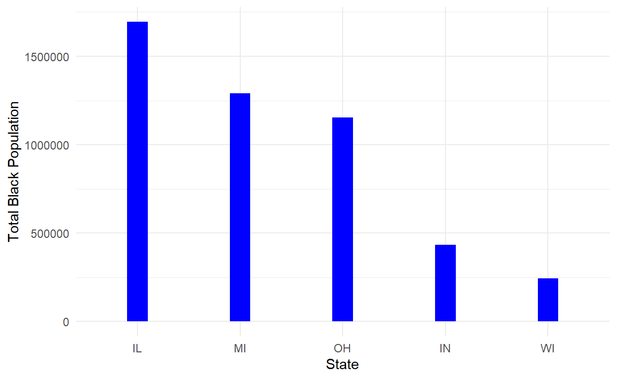

a histogram or density of a continuous variable

# histogram of population density

midwest %>% 
  ggplot(aes(x = popdensity)) + geom_histogram(bins = 10) +
  theme_minimal()+labs(x = "Population Density", y = "Frequency")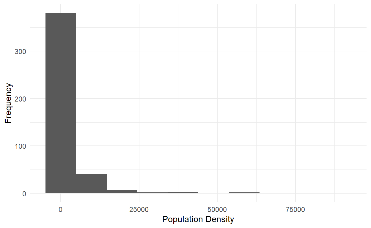

# density

midwest %>% 
  ggplot(aes(x = popdensity)) + geom_density(stat = "density", fill = "green") + labs(x = "Population Density", y = "Density")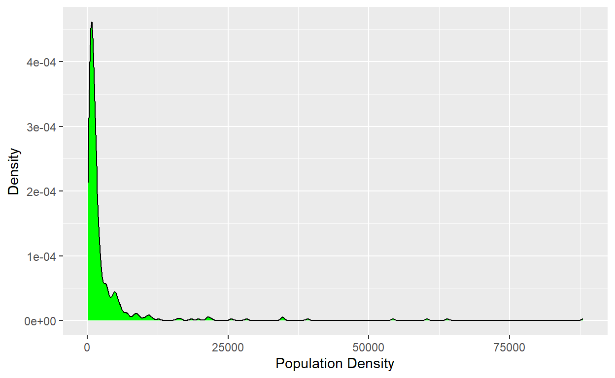

a summary statistic of a continuous variable for each value of a discrete variable

out <- midwest %>% 
  group_by(state) %>% 
  summarize(Mean = mean(poptotal),
            Median = median(poptotal),
            Maximum = max(poptotal), 
            Minimum = min(poptotal))
knitr::kable(out)

state	Mean	Median	Maximum	Minimum
IL	112064.73	24486.5	5105067	4373
IN	60262.60	30362.5	797159	5315
MI	111991.53	37308.0	2111687	1701
OH	123262.67	54929.5	1412140	11098
WI	67941.24	33528.0	959275	3890

# visual representation

midwest %>% 
  ggplot(aes(x=state, y = poptotal)) + geom_boxplot()+ theme_minimal()+
  labs(y = "Population Total")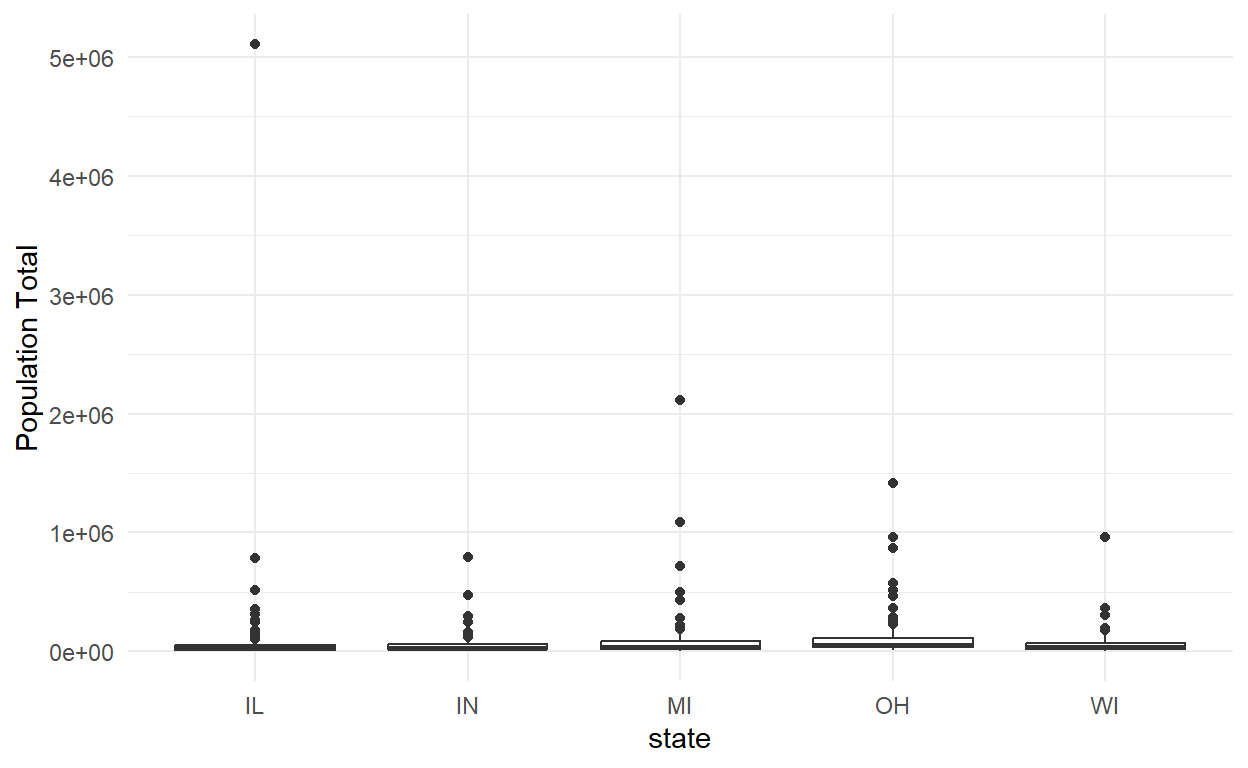

a scatterplot of two continuous variables, with a smoothed conditional mean line.

# we explore poppovertyknown and percollege 

midwest %>% 
  ggplot(aes(x = percollege, y = percbelowpoverty)) + 
  geom_point() + geom_smooth(method = "lm")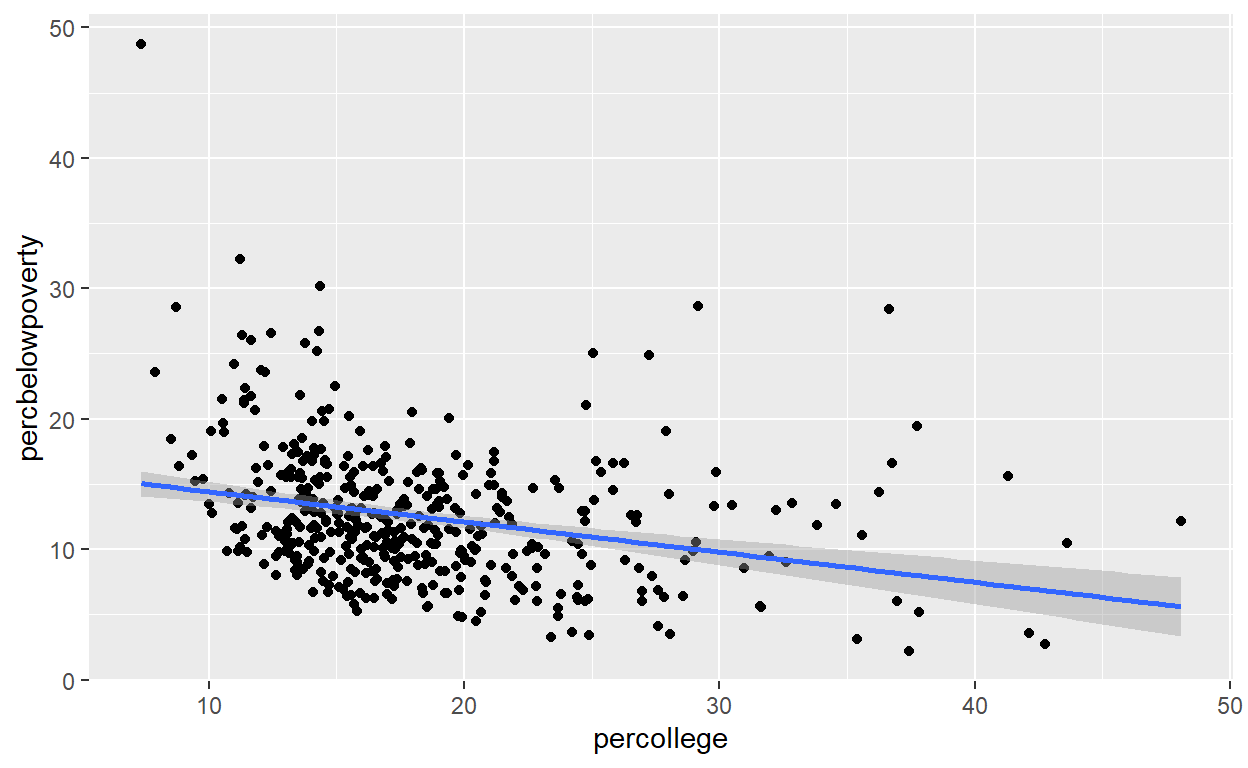

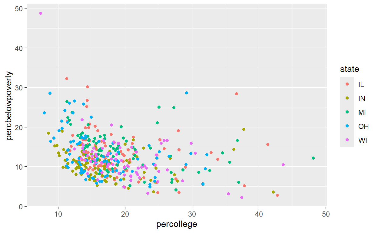
three variables.

midwest %>% 
  ggplot(aes(x = percollege, y = percbelowpoverty,color = state))+
  geom_point()

Solutions